
One of the most common techniques that is used in molecular biology labs to quantify differences in gene expression, microbial abundance, or even diagnose diseases and conditions is quantitative polymerase chain reaction (qPCR)/Real-time PCR. Below, I’m going to discuss the two most common formats that are used in qPCR and how to analyze that raw data once it comes back from the thermal cycler!
SYBR Green vs TaqMan
There are two main methods of detection that are used in qPCR reactions:
- SYBR Green
- TaqMan probes
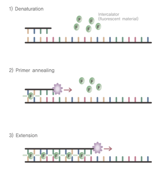
SYBR green is a fluorescent cyanine dye that preferentially binds to double-stranded DNA. Because of this preferential binding, SYBR green is one of the most common ways in which PCR products are detected in qPCR reactions. By measuring the amount of fluorescence throughout the course of the reaction, the buildup of the targeted amplicon can be tracked. However, because SYBR green will bind to any double-stranded DNA, it can occasionally lead to false-positive results.
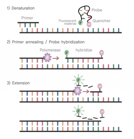
TaqMan probes are hydrolysis probes (oligonucleotides) that have a reporter dye at their 5’ end and a quencher dye on their 3’ end. Typically, the probe is coiled in a way that the dye at the 3’ end inhibits - or “quenches” - fluorescence from the reporter dye. When the sequence of the probe matches a region in the amplicon, the oligonucleotide is incorporated into new double stranded DNA. As the polymerase extends the DNA, the 5’ nuclease activity of the polymerase degrades the probe and releases the reporter dye from the quenching dye. The fluorescence from the reporter dye can then be measured. As more oligonucleotide probes are incorporated into more amplicons, the fluorescent signal increases and can be tracked in real time. While TaqMan probes are typically more specific than SYBR green assays, TaqMan probes must be custom designed for each assay and are more expensive than assays using SYBR green. However, multiple TaqMan probes with reporter dyes that emit at different wavelengths can be used to detect multiple targets in the same reaction (known as multiplexing).
qPCR Thermal Cycler Output
The main data that is used to quantify the amount of a specific target in your qPCR reaction is known as the cycle threshold (CT) value. The CT (also sometimes called Cq) represents the cycle number (typically 1-40) that it took for the measured fluorescence of a sample to cross the detection threshold (the red line below). This detection threshold is typically placed in the middle of the linear phase of the amplification curve, just as it is shown below.
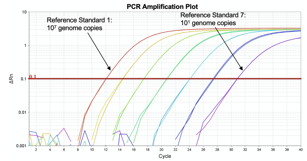
When quantifying the abundance of a specific target in your reactions, it is typical to run multiple known ‘standards’ with a known amount of your target (I typically use custom DNA or RNA oligonucleotides from IDT). These known standards are then used to plot a standard curve based on their CT values and known quantity.
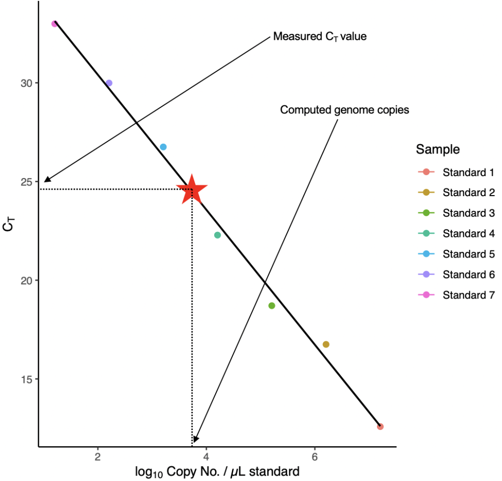 The unknown samples can then be compared (using their CT value) against the plotted standard curve to determine the number of genome copies present in your samples.
We are normally interested in the abundance in hundreds of samples so plotting and determining the abundance in each sample would be time-consuming and low throughput. To get around this, I instead use the R statistical computing environment to process all of my qPCR data. When I receive the raw data from the thermal cycler, it is typically outputted as a .csv file. Although these files will differ based on the brand and model of real-time PCR system that is used, most will contain some combination of this data.
Note: This data was outputted from an Applied Biosystems SteOnePlus instrument. If you run into problems formatting your code/data, feel free to reach out to me at pfh@uoregon.edu for some help!
Background on our Data
If you want to follow along with the data and run it yourself, you can find all of the data and code HERE
The data that we are going to be using for this walkthrough was from a test of a new propidium monoazide (PMA) protocol in our lab. Amplification was monitored using SYBR green using the Total Bacteria F SYBR Primer and Total Bacteria R SYBR Primer (Fahimipour et al., 2018). I’ll be making a separate post about PMA, but in short, PMA helps us differentiate between living and dead bacterial cells in PCR reactions by inhibiting PCR in dead cells. These samples were cultured overnight and split into four experimental conditions:
- Killed w/ isopropyl alcohol + treated w/ PMA (IOH+, PMA+)
- Killed w/ isopropyl alcohol + not treated w/ PMA (IOH+, PMA-)
- Not killed w/ isopropyl alcohol + treated w/ PMA (IOH-, PMA+)
- Not killed w/ isopropyl alcohol + not treated w/ PMA (IOH-, PMA-)
If the PMA treatment worked, we would expect to see similar levels of amplification in all of the treatment groups except for the one treated with both isopropyl alcohol and PMA.
qPCR Data Analysis in R
First, we must bring our data into R, make sure any samples that didnt amplify (they won’t have a CT value) are “NA”, and combine each of the replicates (qPCR is typically run in triplicate):
qp1 <- read.csv(/path/to/file.csv, header = T,skip = 7, stringsAsFactors = F)

qp1[qp1 == "Undetermined"] <- NA

qp1.1 <- qp1 %>%
dplyr::group_by(Sample.Name) %>% #, run) %>%
dplyr::summarise(Ct = mean(as.numeric(as.character(Ct)))) %>%
as.data.frame()
Before we look at our samples, we need to look at our standards and build our standard curve:
# Make an object with just our standards
standards1 <- qp1.1[grepl('Standard', qp1.1$Sample), ]

# Remove the standards from the data set with all the other samples
qp1.1 <- qp1.1[!grepl('Standard', qp1.1$Sample), ]

# Describe our dilution curve and how many gene copies are in each       standard
dil <- c(1,
         .1,
         .01,
         .001,
         .0001,
         .00001,
         .000001)

standards1 <- cbind(standards1, dil)

copy.1 <- c(354287400,
            35428740,
            3542874,
            354287.4,
            35428.74,
            3542.874,
            354.2874)

# Now we can combine everything and make our standard curve
dat1 <- data.frame('Sample'= standards1$Sample, 'copy' = copy.1, 'log.copy' = log10(copy.1), 'Ct' = standards1$Ct)

fit1 <- lm(Ct ~ log.copy, data = dat1)

line1 <- lm(Ct ~ log.copy, data = dat1)

ab1 <- coef(line1)
Now lets take a look at our standards in a plot:
ggplot(dat1, aes(x = log.copy, y = Ct, colour= Sample)) +
  theme_classic() +
  xlab(expression('log'['10']*' Copy No. / µL standard')) +
  ylab(expression('C'['T'])) +
  labs(subtitle = paste("Adj R2 = ",signif(summary(fit1)$adj.r.squared, 5),
                        "Intercept =",signif(fit1$coef[[1]],5 ),
                        " Slope =",signif(fit1$coef[[2]], 5),
                        " P =",signif(summary(fit1)$coef[2,4], 5))) +
  geom_point(size = 2) +
  geom_line(aes(group=as.factor(Sample))) +
  stat_smooth(method = 'lm', formula = y ~ x, level = 0, size = 0.75, col = "black")
This looks great! The biggest thing that I am looking for here is that there is a fairly linear relationship between all of the points of the standards (check!), our R2 value is above 0.96 (check!) and our p value is significant (check!). Everything looks good!
Next, we need to apply this standard curve to all of our samples in order to determine the abundance of our target in each of them! This function will take the standard curve and apply it to our unknown abundance samples:
convert <- function(y, b, a){
  x <- 10^((y - b) / a)
  x
}
Now we can run the actual conversion function:
qp1.1$counts <- convert(y = as.numeric(qp1.1$Ct), b = ab1[1], a = ab1[2])
And these two lines will remove any contaminants introduced by reagents or the PCR prep:
NTC.1 <- qp1.1[grepl('ntc', qp1.1$Sample), ]

NTC.1 <- as.numeric(NTC.1$counts)

NTC.1
[1] 1.458381
Note that there is a very low abundance of our target in the NTC (no template control). Whether or not this is a major problem for your reaction is very much situation dependent. In this case, the abundance in the NTC is ~significantly~ lower than in any of our actual samples. Additionally, because we are quantifying general bacterial abundance, it is unlikely that the NTC would ever be completely clean, simply because we are covered in bacteria ourselves and can introduce bacteria as we prep the reaction! Comparatively, if you are looking for some rare pathogen and find it highly abundant in your NTC, then you may have a cross-contamination problem and should switch out reagents and rerun the samples!
Now we can look at our final data! (Note: the counts observed in the NTC have been removed even though they are still shown below)
qp1.1
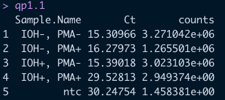
There is clearly a significant drop-off in the detectable abundance of our samples were killed and treated with PMA just as we expected! This is great!
This is definitely not the only way to process qPCR data and likely is not perfect for every application, but it is a fairly standard workflow and is a great starting point! Please do not hesitate to reach out with any questions or concerns!